Mechanical analysis is the determination of the size range of particles present in a soil, expressed as a percentage of the total dry weight. There are two methods generally used to find the particle-size distribution of soil: (1) sieve analysis - for particle sizes larger than 0.075 mm in diameter, and (2) hydrometer analysis - for particle sizes smaller than 0.075 mm in diameter. The basic principles of sieve analysis and hydrometer ever analysis are briefly described in the following two sections.
Sieve analysis consists of shaking the soil sample through a set of sieves that have progressively smaller openings. Table 1 lists the U.S. standard sieve numbers and the sizes of openings.
Table 1. U.S. Standard Sieve Sizes.
Sieve Number |
Opening (mm) |
4 |
4.750 |
6 |
3.350 |
8 |
2.360 |
10 |
2.000 |
16 |
1.180 |
20 |
0.850 |
30 |
0.600 |
40 |
0.425 |
50 |
0.300 |
60 |
0.250 |
80 |
0.180 |
100 |
0.150 |
140 |
0.106 |
170 |
0.088 |
200 |
0.075 |
270 |
0.053 |
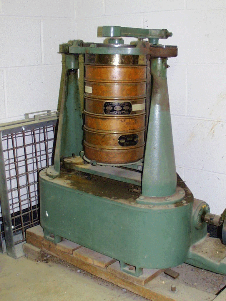
First the soil is oven dried and then all lumps are broken into small particle before they are passed through the sieves. Figure 1 shows a set of sieves in a sieve shaker used for conducting the test in the laboratory. After the completion of the shaking period the mass of soil retained on each sieve is determined. When cohesive soils are analyzed, it my be difficult to break lumps into individual particles. In that case, the soil may be mixed with water to make a slurry and then washed through the sieves. Portions retained on each sieve are collected separately and oven dried before the mass retained on each sieve is measured.
Figure 1. Set of sieves in a sieve shaker
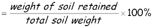
The results of sieve analysis are generally expressed in terms of the percentage of the total weight of soil that passed through different sieves. Table 2 shows an example of the calculations required in a sieve analysis.
Table 2. Sieve Analysis (Mass of Dry Soil Sample = 450 g).
Sieve Number |
Diameter |
Mass of
soil retained |
Percent
of soil |
Percent |
10 |
2.000 |
0 |
0 |
100.00 |
16 |
1.180 |
9.90 |
2.20 |
97.80 |
30 |
0.600 |
24.66 |
5.48 |
92.32 |
40 |
0.425 |
17.60 |
3.91 |
88.41 |
60 |
0.250 |
23.90 |
5.31 |
83.10 |
100 |
0.150 |
35.10 |
7.80 |
75.30 |
200 |
0.075 |
59.85 |
13.30 |
62.00 |
Pan |
-- |
278.99 |
62.00 |
0 |
Hydrometer analysis is based on the principle of sedimentation of soil grains in water. When a soil specimen is dispersed in water, the particles settle at different velocities, depending on their shape, size, weight, and the viscosity of the water. For simplicity, it is assumed that all the soil particles are spheres.
The results of mechanical analysis (sieve and hydrometer analyses) are
generally presented by semi-logarithmic plots known as particle-size distribution curves.
The particle diameters are plotted in log scale, and the corresponding percent finer in
arithmetic scale. As an example, the particle-size distribution curves for two soils are
shown in Figure 2. The particle-size distribution curve for soil A is the combination of
the sieve analysis results presented in Table 2 and the results of the hydrometer analysis
for the finer fraction. When the results of sieve analysis and hydrometer analysis are
combined, a discontinuity generally occurs in the range where they overlap. This is
because soil particles are generally irregular in shape. Sieve analysis gives the
intermediate dimension of a particle; hydrometer analysis gives the diameter of a sphere
that would settle at the same rate as the soil particle.
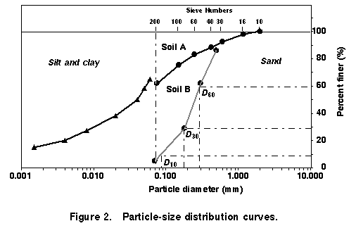
The percentages of gravel, sand, silt, and clay-size particles present in a soil can be obtained from the particle-size distribution curve. According to the Unified soil classification soil A in Figure 2 has:
Weigh to 0.1 g each sieve which is to be used. Make sure each sieve is clean before weighing it.
Select with care a test sample which is representative of the soil to be tested; break the soil into its individual particles with the fingers or a rubber-tipped pestle.
Weigh to 0.1 a specimen of approximately 500 g of oven-dried soil. If the soil to be tested has many particles coarser than the openings in a No. 4 sieve, a larger weight of soil should be used.
Sieve the soil through a nest of sieves by hand shaking. Using a motion of horizontal rotations or using a mechanical shaker, if available. At least 10 minutes of hand sieving is desirable for soils with small particles.
Weigh to 0.1 g each sieve and the pan with the soil retained on them.
Subtract the weights obtained in step 1 from those of step 5 to give the weight of soil retained on each sieve. The sum of these retained weights should be checked against the original soil weight.
If a sizable portion of soil is retained on the No. 200 sieve, it should be washed. This is done by placing the sieve and retained soil in a pan and pouring clean water on the screen. Use a spoon or glass rod to stir the slurry. Recover the soil which is washed through; dry and weigh it. The weight of soil recovered should be subtracted from the weight retained on the No. 200 sieve and added to the weight retained in the pan as determined in step 6.
The method of weighing the sieve plus soil rather then attempting to remove the soil from the sieve for weighing is suggested because it has been found that soil is often lost during the removing. Even using this suggested procedure, be careful to minimize the lose of soil during the sieving.
Step 4 recommends that the sieving consist of approximately 10 minutes of horizontal shaking. A horizontal motion was suggested instead of a vertical one since it has been found more efficient and since less soil escapes from the nest of sieves during horizontal shaking. The amount of shaking required depends on the shape and number of particles. As an example of the fact that the shaking time required is increased as the number of particles is increased, for crushed quartz it was found that, in a given time, the percentage passing was 25% less for a 250-g sample than it was for a 25-g sample. Since a given weight of a fine-grained soil contains more particles than an equal weight of a coarse-grained one, more shaking time is necessary for the finer-grained soils.
Percentage retained on any sieve:
Cumulative percentage retained on any sieve:
Percentage finer than an sieve size:
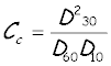
The particle-size distribution curves can be used for comparing different soils. Also, three basic soil parameters can be determined from these curves, and they can be used to classify granular soils. Them parameters are:
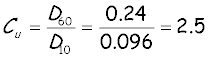
The diameter in the particle-size distribution curve corresponding to 10% finer is defined as the effective size, or D10. The uniformity coefficient is given by the relation:
where Cu is the uniformity coefficient and D60 is the diameter corresponding to 60% finer in the particle-size distribution
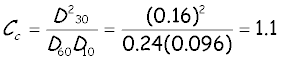
The coefficient of gradation may he expressed as:
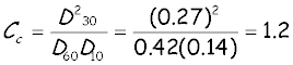
where Cc is the coefficient of gradation and D30 diameter corresponding to 30% finer.
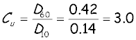
For the particle-size distribution curve of soil B shown in Figure 2, the values of D10 D30 and D60 are 0.096 mm, 0.16 mm and 0.24 mm, respectively. The uniformity coefficient and coefficient of gradation are:
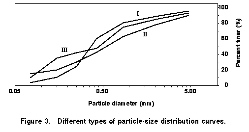
The particle-size distribution curve shows not only the range of particle
sizes present in a soil but also the type of distribution of various size particles. This
is demonstrated in Figure 3. Curve I represents a type of soil in which most of the soil
grains are the same size. This is called poorly graded soil. Curve II represents a soil in
which the particles are distributed over a wide range, termed well graded. A well graded
soil will have a uniformity coefficient greater than about 4 for gravels and 6 for sands,
and a coefficient of gradation between 1 and 3 (for gravels and sands). A soil might have
a combination of two or more uniformly graded fractions. Curve III represents such a soil.
This type of soil is termed gap graded.
From the results of a sieve analysis, shown below, determine: (a) the percent finer than each sieve and plot a grain-size distribution curve, (b) D10, D30, D60 from the grain-size distribution curve, (c) the uniformity coefficient, Cu, and (d) the coefficient of gradation, Cc.
Sieve Number |
Diameter |
Mass of
soil retained |
4 |
4.750 |
28 |
10 |
2.000 |
42 |
20 |
0.850 |
48 |
40 |
0.425 |
128 |
60 |
0.250 |
221 |
100 |
0.150 |
86 |
200 |
0.075 |
40 |
Pan |
-- |
24 |
The following table can be prepared for obtaining the percent finer:
|
Mass of
soil retained |
Percent
retained |
Cumulative
Percent |
Percent |
4 |
28 |
4.54 |
4.54 |
95.46 |
10 |
42 |
6.81 |
11.35 |
88.65 |
20 |
48 |
7.78 |
19.13 |
80.87 |
40 |
128 |
20.75 |
39.88 |
60.12 |
60 |
221 |
35.82 |
75.70 |
24.30 |
100 |
86 |
19.93 |
89.63 |
10.37 |
200 |
40 |
6.48 |
96.11 |
3.89 |
Pan |
24 |
3.89 |
100.00 |
0 |
617 |
The plot of the grain-size distribution is shown below:
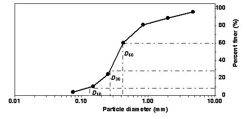
The particle diameters defining 10%, 30%, and 60% finer from the grain-size distribution curve are estimated as: D10 = 0.14 mm , D30 = 0.27 mm, and D60 = 0.42 mm.
This website was originally developed by Charles Camp for his CIVL 1101 class. This site is maintained by the Department of Civil Engineering at the University of Memphis. Your comments and questions are more than welcome.